 The horizontal scale represents values of σ and the vertical scale is probability density.
At a young and impressionable age students are taught how to find the variance (and hence the standard deviation, its square root). The method is to work out the sum of the squares of the deviations of the mean, and then divide by n, the number of objects, to get an average squared deviation from the mean. This is the variance. Students remember this. Then, when they come to University, unkind lecturers tell them that sometimes they should divide by n-1 instead of n. This tends to make the students unhappy. They thought that they knew what they were doing with variances, and now they don't. Most of them don't understand why they need to do anything different from before, which makes it difficult to remember when it is that they are supposed to do it.
Thus I am often asked to explain what is going on with the n-1. I seldom have time to do it properly, so I'm writing down here why we need to use it. It's called Bessel's correction, after Friedrich Bessel, who worked it out.[1] I shall also go on to explain why it isn't, really, the right thing to do in many practical cases, and some alternative approaches. I finish with a problem to which I don't know the answer. But if you just want to know why, how, and when to apply the correction, just read the first two sections.
The first thing to say is that the formula taught at GCSE is correct. If you want to find the variance of a set of numbers, then you should work out the sum of the squared deviations from the mean, and divide it by n. That is the definition of the variance. The problem is that you don't always have all of the numbers. And if you don't have all of the numbers, then you can't work out the exact, true variance. You can only make an estimate of it. The challenge is to make this estimate as good as it can be!
Suppose that we want to find the variance of lengths of tails on rats in the United Kingdom. To work out the exact, true variance, we would need to catch all of the rats in the Kingdom and measure their tails. This is impracticable.[2] Instead, what we'd do is catch a few rats at random,[3] measure their tails, and try to extrapolate. The numbers that we measure on the rats we've caught are the "sample". If it was the true mean tail length that we wanted to find, the right thing to do[4] would be to take the mean of the sample and declare this to be the best estimate. This is just what you might expect. But if it's the true variance that we want to estimate, we shouldn't just find the variance of the sample and declare this to be our best estimate. On average, it will be too small.
Why is this? The problem is that we don't know the true mean: we only have an estimate of it, and this estimate is biased to the numbers that we have in our sample. The deviations that we work out are therefore deviations from the sample mean, not from the true mean. For example, if the rats that we caught had a slightly longer mean tail length than the true population mean, then we'd produce an estimate of the mean that was a bit bigger than the true value. Our deviations would then be smaller (in absolute value) than the true deviations, because the true deviations are those from the true mean, which is a smaller number than the one that we're using and therefore further away on average from the numbers that we have. Likewise, if we've caught shorter-tailed rats than average, we will underestimate the mean. But again this causes us to get deviations smaller than the true deviations, because this time the tails are atypically short, so they're closer to the sample mean than they would be to the population mean. Hence it doesn't matter which sort of rats we've got: the sample variance is always going to tend to be[5] an underestimate of the true variance.
Therefore we need some sort of recipe for taking the sample variance and making it a bit bigger so that we somehow get a better estimate of the true variance. This is what Bessel's correction does.
An intuitive way of thinking about Bessel's correction goes as follows. We started off with n pieces of information, the n pieces of sample data. We have used them to find an estimate of the mean. This effectively uses up one degree of freedom: instead of thinking of it as n random (free) measurements and their (dependent) sample mean, we can think of the sample mean as the actual mean of some distribution (with the same variance as the true one) but with only n-1 measurements' worth of free variation amongst the n readings. Thus we need to correct our estimate by n/(n-1).
The trouble with this argument is that it appeals to a particular sort of intuition that is difficult to make rigorous. A better approach goes as follows. (This is more-or-less just writing out in words the "Alternate 1" from the Wikipedia page on Bessel's Correction.)
A lemma is just a theorem, a mathematical result, whose main purpose is that it's a stepping stone to a more important result. In this case the more important result is Bessel's correction, and the lemma is as follows: for any set of data, the expected value of the squared difference between two randomly chosen values is exactly twice the variance of the data.
To prove this, note that the difference between two values is the same as the difference between their deviations from the mean. Thus instead of finding the expected value of (x1 - x2)2, which is what we want, we can find the expected value of (d1 - d2)2, where d1 = x1 - mean, and d2 = x2 - mean.[6] Hence what we want, multiplying out, is d12 - d1d2 + d22. The expectations of the first and third terms are each the variance of the data, by definition. The expectation of the middle term must be zero, because the expected values of the deviations d1 and d2 are each zero.[7] Thus the total expected value is twice the variance.
It's important to note that the lemma applies to any set of data, whether it's what we've been calling the sample, or what we've been calling the population.
Consider the squared difference between two randomly chosen values in the sample. Most of the time it's the squared difference between two distinct values, which means that it has the same expected value as that equivalent quantity in the population. However, sometimes (1/n of the time, in fact) it's just zero, because we happen to have chosen the same value for x1 and x2. Thus the expected value of the squared difference between values is smaller in the sample than in the population, by a factor, on average, of 1 - 1/n.
Now according to the lemma, the variance is always exactly half of the expected value of the squared difference between values. So the variance of the sample is, on average, smaller than the variance of the population by this same factor 1 - 1/n, which is (n-1)/n. So if what we have is the sample variance, we should multiply by n/(n-1) to get a better estimate of the population variance.
Some of the confusion surrounding this subject is due to the notation used. People sometimes call the standard deviation of a set of numbers the "population standard deviation", and write it as σn. (It is often called σn on calculators. The notation makes sense because, when finding the variance, we divide by n.) They then sometimes refer to the corrected quantity, √(n/(n-1)) times this, the estimate of the true population standard deviation if what we had was a sample, as the "sample standard deviation", and write it as σn-1. The σn-1 notation at least reminds us what we're doing, but calling it the sample standard deviation is potentially confusing, because it's not the standard deviation of the sample. Instead, it's an estimate of the population standard deviation if what we had was a sample.
In more serious work, the true, unknown variance of the population is usually denoted σ2, and the actual variance of the sample is usually denoted s2. Thus what Bessel's correction tells us is that an unbiased estimator for σ2 is given by (n/(n-1))s2. I'll use this notation in subsequent sections. I'll also use μ for the true, unknown mean of the population, and x for the actual mean of the sample.
What we find using Bessel's correction is what is known as an "unbiased estimator". This means that, if we used the same underlying population and took lots of samples, using the estimation technique on each one, then the average of all of the estimates would approach the true value, σ. In other words, the expectation value of the estimate is the true value. This is why we used (effectively) the expectation value of the sample variance in the proof above.
Unbiased estimators sound difficult to argue with. How could bias be a good thing, after all?
There are several problems with using the unbiased estimator for variance. For a start, what we really want to know is probably the standard deviation, not the variance. This doesn't sound like much of a problem: if we know the variance, we can just take the square root to get the standard deviation. But we don't know the variance; we only have an (unbiased) estimate of it. And the square root of that is not, in fact, an unbiased estimate of standard deviation. I've briefly outlined what has gone wrong, and how it can be fixed, in the next section.
There's a more fundamental problem, though: lack of bias doesn't really mean that an estimate is much use. To take an extreme example, suppose that a certain quantity has a true value of 11. Then an estimator that is always 1, except for one time in every million when it is 10000001, would technically be unbiased, because the expected value of the estimator would equal the true value. But it would almost always be an order of magnitude too small. This is a particularly silly example, since we know the true value, so we can give the best possible estimate according to all possible criteria as just being 11, every time. But what is shows is that being unbiased isn't enough to make an estimator useful. A more practical example of this sort of thing is to be found on the Wikipedia page about bias of estimators in statistics. Although requiring estimators to be unbiased seems like a good thing in principle, it doesn't really capture the properties that we really need. I'll address this later on.
Even if we do want an unbiased estimator, the trouble with just taking the square root of the unbiased estimate of the variance is that the square root of an expected value is not the expected value of the square roots. (After all, the mean of 9 and 25 is 17, but the mean of 3 and 5 is 4, which isn't the square root of 17.) Correcting for this problem is inconvenient. The correct approach depends on what the probability distribution actually is, a thing that we didn't need to know in the case of the variance. If we make the assumption that the distribution is Gaussian[8], then we can find the equivalent thing to Bessel's correction, but it's a nasty formula involving the gamma function. It can be approximated, very roughly, by using n-1.5 instead of n-1 in the denominator of the correction. This is all explained in the "bias correction" section of an informative Wikipedia page. [9]
However, as I mentioned above, finding the unbiased estimator needn't be the right way to summarize what we know about the standard deviation.
The most complete statement of what we know about an uncertain quantity is not an estimator, nor is it a selection of estimators flawed in different ways. It isn't even an essay about how well or badly different estimators work in a particular case. The most complete statement of what we know about an uncertain quantity is a probability distribution. We start off with a probability distribution, the prior, that represents the information we have before the experiment. (This will be some sort of uniform prior if we have negligible information before the experiment.) We then update this using the data from the experiment, together with Bayes' theorem, to get the posterior probability distribution.[10] Finding an estimator is really just a way to find a value that summarizes that distribution.
Let's assume that we know nothing about σ before the experiment. But what does it really mean to know nothing? We could say that we think any value equally likely, leading to a uniform prior. But this isn't the right thing to do if we don't even know what order of magnitude a number will have, because according to a uniform distribution a number between 10 and 90 is ten times more likely to occur than a number between 1 and 9. In this case we probably want a log-uniform prior. I'll quote results below for both choices of prior distribution for the standard deviation.[11]
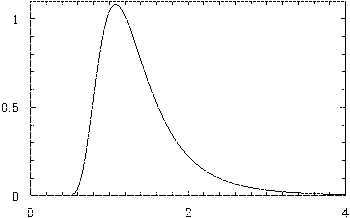
If we assume that the underlying distribution is Gaussian,[12] and use Bayesian analysis to work out the probability distribution for the possible values of σ, we find a distribution which is a transformation of the well-known Chi-squared distribution. I don't want to write out the formula, but the distribution looks something like this.
The horizontal scale represents values of σ and the vertical scale is probability density.
This is the probability density function for σ, given that a sample of n=7 values has s=1, and assuming a uniform prior for the standard deviation. Notice that it isn't symmetrical, but is positively skewed: there is a heavy tail to the right of the maximum, compared to the left. This is what we'd expect, because it isn't possible that σ is less than zero, and it's unlikely that it's very small if s is 1; on the other hand, it is possible that σ is fairly big but that all of the readings in the sample just happen to be clustered together.
The trouble with an asymmetric distribution is that it's difficult to summarize. We could quote the mode, defined as the most likely value, i.e. the maximum of the distribution. This turns out to be, curiously, at the place that Bessel's approximation tells us to look, i.e. at s√(n/(n-1)). On the graph above, it occurs at √(7/6). (The result needs modifying slightly if we assume a log-uniform prior: in this case it turns out that the mode is actually at s.)
The trouble with quoting the mode is that, for this distribution, it's well to the left of the distribution, because of the positive skew. (In the example plotted above, the probability of σ being larger than the mode is about 70%.) What should we use instead? One obvious candidate is the median. This is by definition the value which is in the middle of the distribution in the sense that the probability that it is exceeded is exactly 50%. Unfortunately, there isn't a nice formula for the median of this distribution as there is for the mode. It does, though, imply using a bigger correction factor than Bessel recommends. In the example plotted above, the median is at 1.268, implying a correction factor of 1.268, whereas Bessel's approximation, and the mode, occur at 1.080 = √(7/6).
Another option is to find the mean of the distribution. Because of the positive skew, this is even bigger than the mode. I think that there's a nice formula for it, but since (as explained below) it isn't really the best thing to do, I haven't worked it out. Numerically, for the example plotted above, it occurs at 1.981 or so.
At first sight it might seem surprising that the mean of the posterior distribution isn't the same as the unbiased estimator, as they are both in some sense an expectation value for σ. (For the example above, n=7 and s=1, the unbiased estimate of σ is 1.042.) The reason that they're different is that they are averaging over different sorts of repeats. The mean of the posterior distribution, the one referred to in the previous paragraph, averages over all repeats of the experiment, with all possible values of σ that happen to give the same data. It gives the average value of σ that will produce the data. In contrast, the unbiased estimator gives a quantity which, if averaged over many repeats of the experiment with the same σ, will give the true value of that σ.
Which mean is the right mean? Neither. We're not repeating the experiment[13] in any way. The most complete way to state what we know about σ is to give the whole distribution, and any scheme to summarize it ought to be chosen based on what we happen to want the summary for.
Let's take a step back for a moment: why do we want an estimate of σ, the population standard deviation? In many cases, we're not that interested in it for its own sake, because the variation between numbers is due to experimental error, and the thing that we're actually trying to measure is μ, the mean of the distribution. But we need to find it out because we want to give an estimate of the error in the result that we give. Our best estimate of the actual result, μ is given by the mean of the measurements, x, and then our estimate of the error in that mean is given by our estimate of σ (an estimate of the root-mean-square error on each measurement) divided by the square root of n. (We're allowed to divide by the square root of n because taking several readings tends to make the errors partially cancel out on average. This is a well-known result; I don't want to explain why it works here.)
Thus the thing that we're eventually going to use our estimate of σ to try to find out is, itself, a measure of the width of a distribution: the distribution of possible true means. We shouldn't be worrying about how to summarize the distribution of possible σ. The problem that we should really be tacking, using a Bayesian approach, is the distribution of possible μ.
As last time, let's assume that the data are Gaussian distributed, and use Bayesian methods, this time to find the distribution of possible μ. The probability density function for μ turns out to be proportional to (1 + z2)-(n-1)/2, where z = (μ - x)/s. With a few changes of variable name, this turns out to be a well-known statistical distribution called Student's t-distribution.[14] If we assume a log-uniform prior for σ rather than a uniform one (which, as mentioned above, is probably a better expression of what we think that we know in most cases, and also meshes better with the way that Student's t distribution is used in classical statistics) then the n-1 in the formula is replaced by n.
If we have x=0 and s=1[15], and assume a log-uniform prior for σ[16], then the probability density function becomes proportional to (1 + μ2)-n/2, which, for n=7, looks like this.
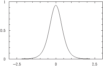 The horizontal scale represents values of μ and the vertical scale is probability density.
It looks fairly similar to the Gaussian distribution, which is not a surprise. In the limit as n goes to infinity it must approach the Gaussian distribution, because of the central limit theorem. But it's slightly different: it has heavier tails, i.e. a larger probability of extreme values relative to its own standard deviation than the Gaussian. (The technical term for this sort of distribution is leptokurtic.) The problem of finding a measure of the expected error in the measurement of μ becomes the problem of characterizing the width of this distribution.
Perhaps the first thing that springs to mind, when looking for a measure of the width of a distribution, is to find its standard deviation. For the distribution above, the standard deviation of μ is 1/√(n-3). (Thus in the specific case n=7 illustrated above, it's exactly 0.5.) If we then work back to what we would have to estimate for σ in order to derive this error in the mean when dividing by √(n), it's equivalent to replacing Bessel's correction by a factor of √(n/(n-3)).
It's nice that the result is so simple and exact, but I think that it's worth asking whether its standard deviation is really the best way to characterize the distribution. When people are given a standard error, they tend to assume that it obeys Gaussian statistics, and this doesn't. So it's perhaps worth looking at how to characterize the width in a way that preserves probabilities compared to the Gaussian distribution.
We know that, for the Gaussian distribution, 68%[17] of the data lie within one standard deviation of the mean. So perhaps one way to quote the standard error in μ would be to quote the +/- value such that μ lies within that range (i.e this distance either side of x) with 68% probability. The problem can be solved numerically. It turns out that the answer (as a +/- value for μ given x=0 and s=1) is approximately 1/√(n-2); it is well approximated by that formula even for n as small as 5, and the approximation gets better as n increases. This is equivalent to replacing Bessel's correction by a factor of √(n/(n-2)).
Somewhat to my annoyance, I can't prove this result, though the numerical evidence for it is very strong. What I want to prove is that if k is defined as satisfying
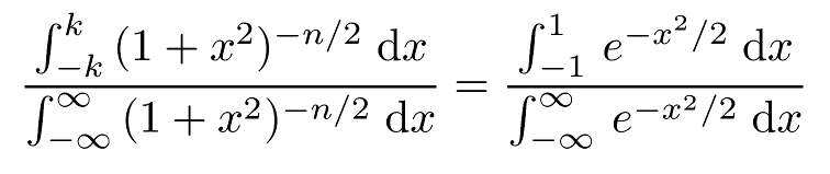
then k-2 = n - 2 + O(1/n). Yes, I can evaluate both of the denominators. I've just left them in integral form to make it clear where the calculation is coming from.
Matching the t-distribution to the Gaussian at the one standard deviation (of the Gaussian) point may not be the right thing to do, though. When interpreting a range of possible results, people perhaps usually make heavier use of the assumption that the probability that the value lies within two standard errors of the mean is 95%[17]. Similar numerical work to that of the last section suggests that Bessel's correction should then be replaced by √(n/(n-3.5)). Again I don't have a proof. (And this time it doesn't become a good approximation until n=10 or so.)
If we need to bring the probability of being wrong down further, say to beyond the 5σ level that CERN insists on before admitting that it's discovered a new particle, we'll need more formulae. At this point the numerical methods that I've been using start to lack sufficient precision!
The result of the last section suggests that we should use n-2, or possibly n-3.5, instead of the n-1 of Bessel's correction. Under the assumptions made, we should. But I've been assuming for several sections that the underlying distribution is Gaussian, and it might not be. (Bessel's correction, on the other hand, is correct on its own, albeit artificial, terms whatever the underlying distribution.) If we really want to use a proper Bayesian approach, which will make the answer as right as it can be, we'll need to incorporate whatever information we have about the underlying distribution. And then, as always, the fullest statement of what we think we know is a probability distribution.
But there is a quick, practical answer to the question of whether we should use n, n-1, n-1.5, n-2, n-3, n-3.5, or something else in simple, everyday cases where working out the full posterior distribution for μ would be excessive. If these numbers are very different from each other, then n is small, so you should take more readings. And then it won't matter very much which you use. Moreover, you'll have a smaller error, and perhaps, even, more idea as to what's going on in your experiment.
Matthew Smith, 2.viii.2014
[1] ^ It appears that he wasn't the first to do so, and that it was first used by Gauss. But Gauss invented practically everything, and we can't name it all after him, or it gets too confusing.
[2] ^ It's at moments like these that the excellent "What If?" articles insert something like [citation needed].
[3] ^ The major challenge would be ensuring that the rats really are randomly chosen, i.e. that the catching process doesn't somehow favour larger or smaller rats. In practice this is likely to be a bigger problem than whether we do or don't use Bessel's correction. But it's one that I'm happy to leave to the biologists.
[4] ^ This is the right thing to do, anyway, if we assume a uniform prior for the underlying mean of the population. Everything becomes much more horrible if we don't.
[5] ^ It's not always going to be an underestimate: sometimes, by chance, the individuals chosen will be significantly more scattered than the general population, and it will be an overestimate. But the point is that it is biased towards being an underestimate on average. In what sense I mean "on average" is to be explored later on.
[6] ^ I'm using x1 and x2 as the two randomly-chosen values. Hopefully this is clear.
[7] ^ I'm using, implicitly, some technical results about combining expectation values here: firstly that we can add them up, and secondly that, provided that the variables are uncorrelated, we can multiply them. These results may make intuitive sense. At any rate they can be proved.
[8] ^ The Gaussian distribution and the normal distribution are two names for the same thing. In statistics generally the name normal distribution is more common. But physicists of a Bayesian persuasion tend to call it the Gaussian distribution.
[9] ^ The other half of that page is taken up by the effect of serial correlation. I'm assuming throughout these notes that the sample data are all purely random selections from the population. (As with the rats.)[3] But in real life serial correlation is an effect to watch out for: it may well be much more important than whether we use Bessel's correction or not!
[10] ^ This is the method of Bayesian inference. I'm rather keen on it, though not everyone agrees.
[11] ^ Whichever prior we assume for the underlying standard deviation, I'll assume a uniform prior for the underlying mean. There are sometimes good theoretical reasons for doing this. In principle we oughtn't to use improper priors (prior distributions like the uniform distribution that can't be normalized), but should instead incorporate such information as we have, however limited it may be, in the form of a cut-off. Otherwise we get all kinds of problems. However, using an un-normalized uniform prior still leads to a normalizable posterior distribution, and the answer is fairly insensitive to where we put the cut-offs provided that they really are well away from the data.
[12] ^ This is a key assumption, and it may not be a good one. We should look at the problem at hand and see what we know about the underlying distribution rather than just assume that it's Gaussian. However, if we want to look at how Bessel's approximation might have to be modified, we will need to focus on a specific example, and the Gaussian distribution is the best example to choose, because it's one that often occurs in the analysis of real experimental errors, it's relatively simple to analyse, and it allows us to make comparisons with standard results from classical statistics.
[13] ^ If we were repeating the experiments, we'd just combine our results and have a larger sample size. That larger sample is then what we should analyse, rather than artificially chopping our results into pieces based on when we happened to take them.
[14] ^ The variable t that appears in the usual form of Student's t distribution differs from my z by a factor of √(ν), where ν is the number of degrees of freedom, equal to n-1.
[15] ^ If we have any other values for x and s, we can just shift and re-scale the answers. And I shall.
[16] ^ I'll do this for the rest of this section. I know that it's inconsistent with the graphical example in the previous section, but I don't want to go back and change it now!
[17] ^ It's really 68% and a bit for one standard deviation, and 95% and a bit for two standard deviations. I'm just writing them to the nearest whole percentage point for brevity.